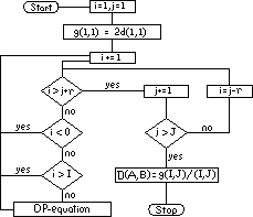
Figure 1. SDP Flowchart
SDP creates a common time axis for two waveforms with differing time axes.
Fuzzy Logic
Fuzzy Logic Enhanced Symmetric Dynamic Programming for Speech Recognition
|
Patrick Mills University of South Carolina Electrical and Computer Engineering Columbia, SC 29208 pmills@ieee.org |
John Bowles University of South Carolina Electrical and Computer Engineering Columbia, SC 29208 bowles@ece.sc.edu |
A PDF version is also available. (238K)
For more information, download the Thesis this work is based upon.
Publiction Information:
Patrick Mills and John Bowles. "Fuzzy Logic Enhanced Symmetric Dynamic Programming for Speech Recognition." Proceedings of the 5th IEEE International Conference on Fuzzy Systems. (New Orleans, LA. September 1996).
Abstract - Fuzzy logic allows effective decision making in the presence of uncertainty. Identifying spoken words, even in an ideal environment by a trained speaker, is a complex task filled with uncertainty. The speech waveform is nonlinear and variant, removing the possibility of simple analysis. Dynamic programming is a time normalization technique that allows static templates to be used to identify spoken words. Fuzzy logic enhancements enable the technique to handle noise and quantization errors better and improves classification accuracy. An important consequence of using a fuzzy based system is that the system's confidence in its identification can be used to accept the identification or to request further information.
1. Introduction
Speech is a human's most efficient communication modality. Beyond efficiency, humans are comfortable and familiar with speech. Other modalities require more concentration, restrict movement, and cause body strain due to unnatural positions. [LEA80]
The main problem in speech recognition, as with other complex tasks that require some form of intelligence, is the amount of information that must be examined before making a classification or decision. Speech recognition is an extremely complex pattern matching problem. The complexity arises from the variability in speech rate, pitch, volume, and emotion. Together with the natural differences in individual human voice production systems, these factors produce a variable and nonlinear waveform. As if these challenges were not enough, a speech recognition system must also deal with non-speech sounds and environmental noise.
Given two representations of the same spoken word by the same speaker under similar conditions, it is highly probable that they will be of different lengths. The main problem is that variations in speaking rate cause nonlinear changes on the time axis. Dynamic Programming (DP) is one technique that attempts to optimally eliminate timing differences between two waveforms.
2. Dynamic Programming
The DP algorithm works by warping one waveform onto the axis of the other. However, rather than merely stretching or compressing the waveform, the algorithm attempts to match the waveforms so that similarities are maintained and time aligned. In the classic algorithm, one of the waveforms is warped onto the time axis of the other. However, recent research has shown that mapping both waveforms onto a new common axis performs much better. This technique is called symmetric dynamic programming (SDP). The flowchart for SDP is shown in Figure 1 for two waveforms, A and B, having I and J samples respectively. [WAIB90, pp. 159 - 163]

Figure 1. SDP Flowchart
SDP creates a common time axis for two waveforms with differing time axes.
The performance of the DP-equation for SDP depends on the chosen slope restriction. The slope restriction ensures that the warping function has an even gradient. It also ensures that the algorithm does not focus on similarities that are outside a window of usefulness. Experimental results show a slope restriction of one to be optimal. Therefore, the DP-equation is: [WAIB90, p. 163]

where the distance between any two samples is given by:
![]()
The DP-equation g(i, j) involves picking the path with the lowest distance and can therefore be viewed as a gradient. With a slope restriction of one, three paths must be examined as shown in Figure 2. The slope restriction requires that the function step at most once in the horizontal or vertical direction before stepping orthogonally or diagonally.
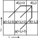
Figure 2. Gradient Paths
When the slope restriction is set to one, three paths must be examined to find the minimum gradient.
The total distance between the waveforms is given at the end of the algorithm as D(A, B). This distance can be used directly as a comparison between the input waveform and a stored template. Alternatively, the common axis representation of the waveform after warping can be used for further processing.
While finding the best time alignment between a template and an unknown, dynamic programming also isolates and matches features. The implementation employed for this paper used dynamic programming on time-amplitude values only; no spectral analysis was performed. While neglecting spectral information limits the overall accuracy of the recognition process, dynamic programming without specialized hardware is too time consuming to perform additional complex analysis such as Fourier analysis or Linear Predictive Coding.
Dynamic programming has a complexity of O(n²), which can cause unreasonable demands on both processing time and system memory. Fortunately, several constraints can be employed to reduce the complexity. By providing a slope constraint, the search area can be limited. Based on work by Sakoe and Chiba, an optimal slope constraint of one was chosen. [WAIB90, pp. 159-65] Dynamic programming can be viewed graphically as a plot of the template waveform (a) vs. the unknown waveform (b). The warping function defines the optimal path from the starting point, which is always (0, 0), to the ending point, (A-1, B-1) where A and B are the lengths of the template and the unknown waveforms respectively. When the two waveforms are exactly the same, the warping function becomes the diagonal line b = a.
Since the starting and ending points are fixed and the slope is constrained, it is possible to define the area of all possible solutions.
| The top and left sides are bounded by: |
The bottom and right sides are bounded by: |
Figure 3 shows the possible paths that may be taken by the warping function. However, due to the recursive nature of the dynamic programming algorithm (equation 1), the left and bottom boundaries cannot be utilized since values outside their boundaries may be needed for calculating values within the area of possible solutions. Notice that the top and right boundaries correspond to starting at the end point and following the lines of maximum and minimum slope towards the starting point. Similarly, the bottom and left boundaries correspond to following the lines of maximum and minimum slope from the starting point and moving towards the end point.
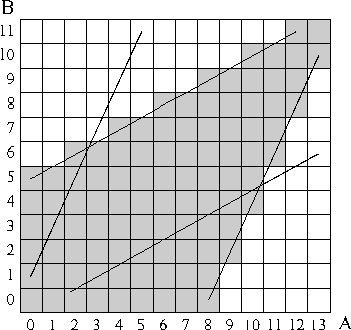
Figure 3. Area Searched by DP Algorithm
The four lines bound the region of all possible solutions. The gray region shows the area that must be searched for possible solutions.
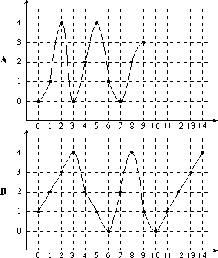
Figure 4. SDP Example
The two waveforms A and B used in the example are shown.
The DP-algorithm is perhaps best explained with an example. Figure 4 shows the two waveforms to be compared; waveform A has a length of 10, and waveform B has a length of 15. The first step is to calculate the distance from each point in waveform A to each point in waveform B. To illustrate the calculations at time 0, B is 1 and A is 0; hence, (0, 0) is 1-0 = 1 in Table 1. At time 1, A is 1; hence, (0, 1) is 1-1 = 0. Table 1 shows the results of these distance calculations. The next step is to apply equation 1 and calculate the recursive gradients as shown in Table 2. The final step is to normalize the gradient at (A-1, B-1) = (9, 14) by dividing by A+B = 25. The final result, 0.36, is the best distance between the two waveforms.
| B \ A | 0 | 1 | 2 | 3 | 4 | 5 | 6 | 7 | 8 | 9 |
| 14 | 4 | 2 | 1 | |||||||
| 13 | 1 | 2 | 3 | 1 | 0 | |||||
| 12 | 2 | 0 | 2 | 1 | 2 | 0 | 1 | |||
| 11 | 0 | 3 | 1 | 1 | 3 | 0 | 1 | 1 | ||
| 10 | 0 | 1 | 4 | 0 | 2 | 4 | 1 | 0 | 2 | |
| 9 | 1 | 0 | 3 | 1 | 1 | 3 | 0 | 1 | ||
| 8 | 4 | 3 | 0 | 4 | 2 | 0 | 3 | 4 | ||
| 7 | 2 | 1 | 2 | 2 | 0 | 2 | 1 | |||
| 6 | 0 | 1 | 4 | 0 | 2 | 4 | 1 | |||
| 5 | 1 | 0 | 3 | 1 | 1 | 3 | ||||
| 4 | 2 | 1 | 2 | 2 | 0 | 2 | ||||
| 3 | 4 | 3 | 0 | 4 | 2 | |||||
| 2 | 3 | 2 | 1 | 3 | 1 | |||||
| 1 | 2 | 1 | 2 | 2 | ||||||
| 0 | 1 | 0 | 3 |
| B \ A | 0 | 1 | 2 | 3 | 4 | 5 | 6 | 7 | 8 | 9 |
| 14 | 16 | 9 | ||||||||
| 13 | 10 | 15 | 9 | 8 | ||||||
| 12 | 6 | 8 | 11 | 12 | 8 | |||||
| 11 | 3 | 6 | 6 | 9 | 12 | 8 | 9 | |||
| 10 | 0 | 4 | 8 | 4 | 7 | 12 | 8 | 9 | ||
| 9 | 2 | 8 | 5 | 4 | 5 | 10 | 9 | 8 | ||
| 8 | 8 | 5 | 2 | 6 | 9 | 7 | 10 | |||
| 7 | 4 | 2 | 4 | 9 | 7 | 9 | 14 | |||
| 6 | 0 | 4 | 8 | 7 | 9 | 18 | ||||
| 5 | 2 | 4 | 7 | 10 | 11 | 15 | ||||
| 4 | 4 | 10 | 8 | 10 | 10 | |||||
| 3 | 8 | 11 | 6 | 10 | 10 | |||||
| 2 | 6 | 5 | 5 | 9 | ||||||
| 1 | 4 | 4 | 4 | 6 | ||||||
| 0 | 2 | 0 | 6 |
The symmetric dynamic programming algorithm has been implemented in two forms: a classical, crisp form and a fuzzy form. The crisp form calculates the distance at each step by taking the absolute magnitude of the difference between the amplitudes of the two waveforms. The total distance measure between the two waveforms is then given by the sum of these differences divided by the sum of the lengths of the waveforms. This final normalization is necessary so that short waveforms and long waveforms have a common distance measure. The best match is chosen by selecting the waveform with the shortest total distance. The next section discusses the fuzzy implementation.
3. Fuzzy SDP
The fuzzy implementation assumes that all waveforms contain uncertainty. This uncertainty comes from speaker variation, waveform quantization, noise, and the inability to completely specify the process of speech recognition. Each amplitude is therefore represented as a fuzzy number. A fuzzy number may be viewed as a set of numbers around a certain interval. For example, integers close to x can be represented by a fuzzy set in which the closer a number is to x, the higher its membership in the fuzzy set. The fuzzy set must be normal, since x must have maximum membership. [KLIR95]
During the distance calculation, amplitudes are assumed to vary by some specified amount from the measured values. Various values were tested, but a maximum of 16 was experimentally determined to give the best results. Therefore, when the absolute magnitude of the distance between two points is computed, it is adjusted to be a maximum of 16 points closer. The minimum is 0. The membership function, shown in Figure 5, is:

For distances below the fuzzy distance threshold, in this case 16, the degree of membership is computed on the interval [0.5, 1]. For distances above the threshold, the degree of membership linearly decreases to zero as the distance approaches the maximum.
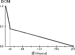
Figure 5. Fuzzy Number Membership Function
Values closer to the actual value have a higher degree of membership, while values further away have lower membership.
The membership of the total distance is the average of the degree of membership of every point along the optimal path. The result of comparing each template to the unknown waveform is a fuzzy set consisting of the set of templates and their degrees of membership, which represent the templates' similarity to the unknown waveform. To defuzzify the result and select the most likely category, the maximum degree of membership is identified. Then the element from the set of maximum membership with the minimum distance is selected as the best match.
4. System Configuration
The majority of isolated word recognizers use a process called template matching to perform recognition. [LEA80] When an unknown waveform is presented to the system, it is compared to a template for each word in the system to find the best match. If found, that template's name is assigned to the unknown waveform. [FRIE68]
Although the recognition system designed for this paper can perform general word recognition, it was designed primarily to perform isolated digit recognition. Since the digits are relatively short, the unit of recognition is a word.
Multiple tests were conducted to determine the system's performance under various conditions. In each test, templates and samples were recorded using a low-cost unidirectional microphone in a noisy environment. The sampling frequency was 6 kHz with 8 bits per sample.
After recording a template or unknown waveform, the system performs segmentation to isolate the word. Various threshold values used by the segmentation routine were tested. The threshold maximum determines how loud a sample must be to indicate the start or end of the word. When processing the waveform, the segmentation routine searches for the first sample that exceeds the threshold. The threshold minimum determines how loud a sample must be to be considered part of the word. Once the threshold maximum is found, the routine searches backward until a sample below the minimum is found. The isolated word is then normalized and stored in memory.
Initial tests were conducted to test the usefulness of removing the waveform's phase and clipping sample values below a specified threshold. In both cases, the system suffered from reduced discrimination. [MILL95]
5. Initial Trial
The first trial was performed using a trained male speaker. The threshold maximum was set to 16, and the threshold minimum was set to 4. Template waveforms for each of the ten digits were recorded and saved first. Then for each digit, ten sample waveforms were recorded and saved. The system was then setup to analyze all 100 "unknown" waveforms using first the crisp classification algorithm and then the fuzzy classification algorithm. The results are shown in Table 3.
| Crisp | Fuzzy | |||
| Digit | % Correct | Error | % Correct | Error |
| 0 | 0 | 3.41 | 80 | 0.74 |
| 1 | 20 | 1.21 | 40 | 0.25 |
| 2 | 20 | 1.88 | 90 | 0.17 |
| 3 | 0 | 3.80 | 30 | 0.71 |
| 4 | 0 | 3.28 | 90 | 0.34 |
| 5 | 0 | 4.68 | 40 | 0.80 |
| 6 | 0 | 4.24 | 100 | 0.0 |
| 7 | 90 | 0.05 | 100 | 0.0 |
| 8 | 0 | 3.34 | 20 | 1.08 |
| 9 | 10 | 1.49 | 100 | 0.0 |
| Total | 14 | 2.75 | 69 | 0.41 |
Error values represent the average distance from the correct classification to the actual classification. Error values were calculated by averaging the absolute magnitude of the differences between the distance from the correct classification and the distance from the actual classification:

where Ei is the Error for digit i, d' is the distance to the correct classification for digit i and d is the distance to the actual classification made by the system for digit i.
Analysis of the crisp results revealed that when the system misclassified a waveform, it classified it as the waveform Six 83% of the time. Examination of the templates revealed that the waveform for Six was on average 2.25 times shorter than the other templates. Even though distance calculations are normalized to reduce the effects of template length, an extremely short template, relative to the lengths of the other templates, will predispose the system to that classification. The fuzzy results show a more even distribution among misclassifications.
The waveform for the template Six was much shorter than the other templates because it begins and ends with the unvoiced phoneme s. Unvoiced phonemes have a much lower relative volume than voiced phonemes. Since the threshold maximum was set to a relatively high value, the beginning and ending phoneme were almost completely removed from the template. In order to remove the classification bias, a much lower threshold maximum needs to be used.
6. Additional Trials
Using the same trained male speaker as in the initial trial, a new set of template and sample waveforms were recorded. The threshold maximum was set to 8, and the threshold minimum was set to 0. The results are shown in Table 4.
| Crisp | Fuzzy | |||
| Digit | % Correct | Error | % Correct | Error |
| 0 | 100 | 0.0 | 100 | 0.0 |
| 1 | 60 | 0.29 | 100 | 0.0 |
| 2 | 40 | 0.55 | 100 | 0.0 |
| 3 | 0 | 1.32 | 40 | 0.52 |
| 4 | 10 | 1.56 | 30 | 1.27 |
| 5 | 20 | 1.66 | 70 | 0.28 |
| 6 | 100 | 0.0 | 100 | 0.0 |
| 7 | 0 | 2.81 | 100 | 0.0 |
| 8 | 100 | 0.0 | 100 | 0.0 |
| 9 | 20 | 1.10 | 80 | 0.14 |
| Total | 45 | 0.93 | 82 | 0.22 |
| Crisp | Fuzzy | |||
| Digit | % Correct | Error | % Correct | Error |
| 0 | 100 | 0.0 | 100 | 0.0 |
| 1 | 100 | 0.0 | 100 | 0.0 |
| 2 | 100 | 0.0 | 100 | 0.0 |
| 3 | 100 | 0.0 | 100 | 0.0 |
| 4 | 100 | 0.0 | 100 | 0.0 |
| 5 | 100 | 0.0 | 100 | 0.0 |
| 6 | 100 | 0.0 | 100 | 0.0 |
| 7 | 100 | 0.0 | 100 | 0.0 |
| 8 | 100 | 0.0 | 100 | 0.0 |
| 9 | 100 | 0.0 | 100 | 0.0 |
| Total | 100 | 0.0 | 100 | 0.0 |
The results show a dramatic increase in accuracy for the crisp algorithm. Classification accuracy of all waveforms except Three and Seven increased. Interestingly, recognition for Seven dropped from 90% to 0%; this result is quite unexpected since seven is a two syllable word and has one of the most unique and consistent waveforms. It is interesting to note that the template for Zero was longer than the template for Four (Two was the shortest template).
Another trial was conducted with an untrained female speaker. The segmentation thresholds were the same as with the previous male speaker. The results are shown in Table 5. The system correctly classified all 100 waveforms using both the crisp and fuzzy algorithms.
In an attempt to explain the perfect results of the female speaker, crisp template correlations for each speaker were calculated. The results for the male speaker are shown in Table 6; the results for the female speaker are shown in Table 7. The template correlations are symmetric.
| Digit | 0 | 1 | 2 | 3 | 4 | 5 | 6 | 7 | 8 | 9 |
| 0 | 0 | 11.7 | 14.8 | 13.2 | 12.0 | 13.1 | 15.6 | 13.4 | 14.1 | 16.0 |
| 1 | 0 | 13.9 | 11.2 | 11.7 | 10.7 | 14.3 | 9.9 | 13.3 | 12.5 | |
| 2 | 0 | 12.6 | 15.2 | 12.5 | 15.5 | 15.2 | 13.7 | 12.6 | ||
| 3 | 0 | 11.0 | 10.1 | 13.4 | 12.1 | 10.1 | 11.4 | |||
| 4 | 0 | 11.0 | 12.1 | 10.3 | 9.4 | 14.5 | ||||
| 5 | 0 | 10.0 | 10.8 | 9.0 | 12.5 | |||||
| 6 | 0 | 11.7 | 7.5 | 16.5 | ||||||
| 7 | 0 | 11.9 | 13.0 | |||||||
| 8 | 0 | 10.8 | ||||||||
| 9 | 0 |
| Digit | 0 | 1 | 2 | 3 | 4 | 5 | 6 | 7 | 8 | 9 |
| 0 | 0 | 10.0 | 8.5 | 9.2 | 11.4 | 7.6 | 10.3 | 8.3 | 11.8 | 10.4 |
| 1 | 0 | 9.4 | 9.5 | 14.1 | 7.0 | 7.2 | 6.5 | 10.1 | 8.1 | |
| 2 | 0 | 5.9 | 13.9 | 8.4 | 9.1 | 9.7 | 11.8 | 12.2 | ||
| 3 | 0 | 13.4 | 12.6 | 10.2 | 11.9 | 12.6 | 16.0 | |||
| 4 | 0 | 13.3 | 14.7 | 14.3 | 18.3 | 17.6 | ||||
| 5 | 0 | 11.5 | 10.7 | 8.7 | 8.9 | |||||
| 6 | 0 | 6.5 | 6.5 | 11.6 | ||||||
| 7 | 0 | 7.9 | 9.4 | |||||||
| 8 | 0 | 10.4 | ||||||||
| 9 | 0 |
The correlation results, while interesting, do not provide any revealing answers to the question of why the female speaker's results were so impressive. On average, the male speaker's templates were more diverse, which should indicate that they would be better for classification. One possible answer is that the female speaker was British, which may predispose her to speak clearly and accurately. More trials are needed to determine which factors most prominently affect the system.
7. Sub-Sampling Trials
Using the templates and a subset of the sample waveforms from the initial trial set, sub-sampling trials were performed to determine how well the crisp and fuzzy algorithms respond to information loss. Given a waveform recorded at a specific sampling frequency, sub-sampling involves finding the maximum (or peak) value from a group of samples within a specific time period. For example, the template and sample waveforms were sampled at 6 kHz. Sub-sampling at 1000 Hz involves finding the maximum value from every 6 samples; sub-sampling at 100 Hz means taking the maximum value from every 60 samples. Table 8 shows the results of sub-sampling.
The crisp system tends to be erratic and the results are not consistent as the degree of information loss increases. The fuzzy system is much more tolerant to information loss, and degrades well. These results were expected, and confirm the assertion that fuzzy systems are able to work effectively even in the presence of uncertainty.
| Sub-Sampling | Crisp | Fuzzy |
| Frequency (Hz) | % Correct | % Correct |
| 1000 | 20 | 75 |
| 400 | 10 | 50 |
| 200 | 35 | 45 |
| 100 | 35 | 25 |
8. Conclusions
Analysis of the recognition technique presented here reveals that the use of fuzzy logic enhances the capabilities of a speech recognition system with little additional cost in either hardware or performance. For the male speaker, the fuzzy system performed considerably better than the crisp system. The results also showed that the fuzzy system degraded better than the crisp system as the information's uncertainty increased.
The ultimate goal of speech recognition is the design of a system capable of recognizing continuous speech from multiple speakers from a large vocabulary. Testing speakers using templates from other speakers should provide results that will aid in extending the system's ability to recognize speech from multiple speakers. In addition, clustering algorithms can be used to determine optimal templates for each word in the vocabulary and various segmentation threshold values should be tested to determine optimal levels for general recognition.
References
[DEMO83] De Mori, Renato. Computer Models of Speech Using Fuzzy Algorithms. Plenum, 1983.
[FRIE68] Friedman, David H. Detection of Signals by Template Matching. Johns Hopkins University Press, 1968.
[KLIR95] Klir, George J., and Bo Yuan. Fuzzy Sets and Fuzzy Logic: Theory and Applications. Prentice-Hall, 1995.
[LEA80] Lea, Wayne A., ed. Trends in Speech Recognition. Prentice-Hall, 1980.
[MILL95] Mills, Patrick M. "Fuzzy Speech Recognition." Thesis. University of South Carolina, 1995.
[WAIB90] Waibel, Alex and Kai-Fu Lee, ed. Readings in Speech Recognition. Morgan-Kaufmann, 1990.
Return to Main Page | Return to Fuzzy Logic Page
Contact me at: pmills@ieee.org - © 1995 - 2021 Patrick M. Mills. All Rights Reserved.